Renormalization in QFT with a few examples
Renormalization is the process of relating the parameters in a quantum field theory to quantities we actually measure. It also explains why the effective strength of an interaction changes with the energy scale at which we probe it.
The apparent complication is that quantum fields fluctuate at every wavelength. When we calculate how these fluctuations affect a particle’s mass or interaction strength, we encounter integrals that can diverge.
1. Why divergences appear
Consider a real scalar field with a quartic interaction:

Here  and
 are bare parameters—the parameters appearing in the regulated theory before we match it to observations.
At the classical, or tree, level, these parameters determine the particle mass and scattering strength. Quantum mechanically, loop diagrams modify both.
For example, the one-loop correction to the scalar mass contains an integral proportional to
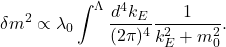
We have written this in Euclidean momentum and imposed a cutoff  . At large momentum,
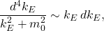
so the integral grows quadratically with the cutoff:

The key point: the bare mass alone is not the measured mass. The measured mass includes the effects of quantum fluctuations.
2. What renormalization does
We rewrite the bare theory in terms of renormalized parameters and counterterms:

The counterterms absorb the regulator dependence of the loop corrections. We then specify renormalization conditions that tell us what  and
 mean.
For example:
- Define the physical mass through the pole of the full propagator.
- Define the interaction strength through a scattering amplitude at specified momenta.
Once these inputs are fixed, the theory predicts other observables.
This involves three distinct steps:

A regulator makes intermediate expressions meaningful. Renormalization makes their connection to measurements precise.
3. Example: mass renormalization in  theory
A free particle has propagator
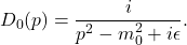
Including quantum corrections gives, with a conventional definition of the self-energy  ,

The physical mass  is determined by the pole:

Thus,

Both the bare mass and the loop correction depend on the regulator. Their combination is fixed by the observed mass.
Physical meaning: the mass of a quantum particle reflects its interactions with quantum fields, as well as the mass parameter in the Lagrangian.
The one-loop quadratic divergence shown earlier is specific to a cutoff treatment; other regulators display the divergence differently. The measured mass cannot depend on that choice.
4. Example: electric charge renormalization in QED
In QED, a photon can fluctuate into a virtual electron–positron pair and back. This produces the vacuum polarization correction to the photon propagator.
Consequently, the electromagnetic interaction measured at one momentum scale differs from that measured at another.
For one active charged Dirac fermion of unit charge, the leading running is
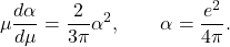
Integrating gives
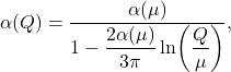
in the regime where this particle content and perturbative approximation apply.
Because the denominator decreases as  increases,

An intuitive picture is screening: vacuum polarization screens electric charge at long distances. Probing shorter distances reveals a stronger effective interaction.
This is an observable consequence of renormalization, beyond removing divergences.
5. Example: running coupling in theory
The four-point scattering amplitude also receives loop corrections. Its divergent part can be absorbed into the quartic coupling.
For a single real scalar field with interaction  , the one-loop beta function is

Therefore,

at this order.
For positive , the coupling grows with energy.
The arbitrary scale  enters when we define the renormalized coupling. A physical scattering amplitude cannot depend on this arbitrary choice. Its explicit logarithmic dependence on cancels against the scale dependence of
 , to the accuracy of the calculation.
6. Example: QCD and asymptotic freedom
QCD shows the opposite behavior. For  active quark flavors,

For the physically relevant numbers of quark flavors, the coefficient in parentheses is positive, so

This is asymptotic freedom.
The crucial difference from QED is that gluons themselves carry the charge associated with the interaction. Their self-interactions produce an antiscreening contribution that dominates the quark screening contribution.
That is why high-energy quark scattering can be treated perturbatively even though low-energy strong-interaction physics is strongly coupled.
7. The deeper viewpoint: physics depends on resolution
In the Wilsonian picture, we imagine integrating out fluctuations with momenta above a chosen scale. Their effects remain encoded in the parameters and operators of the lower-energy theory:
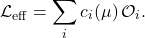
Changing the resolution changes the coefficients  , while preserving predictions for the low-energy processes the theory describes.
This also explains the distinction between:
- Renormalizable theories: a finite set of parameters suffices to absorb ultraviolet divergences, order by order in perturbation theory.
- Effective field theories: additional operators are needed, but only finitely many contribute at any specified accuracy in a low-energy expansion.
Renormalization therefore tells us both how measured parameters incorporate quantum fluctuations and how the description of physics changes with scale.
Leave a Reply