Schrödinger’s Space-Time Structure - Chapter 1 - Time Travel, Quantum Entanglement and Quantum Computing

Let’s work through Erwin Schrödinger’s Space-Time Structure one chapter at a time, explaining both the argument and the mathematics.

The book’s overall approach

Schrödinger builds spacetime geometry in three stages:

Stage	Structure introduced	What becomes possible
Unconnected manifold	Points, coordinates, vectors and tensors	Express local quantities independently of coordinates
Affinely connected manifold	A connection	Differentiate vector fields, transport vectors, define curvature and geodesics
Metrically connected manifold	A metric compatible with the connection	Measure intervals and develop Einstein’s spacetime geometry

His strategy is to identify how much structure each mathematical idea actually requires. For example, tensors can exist before we introduce any notion of distance.

The Introduction also presents his ambition to describe physics geometrically. This is the motivation for the later discussion of unified theories; ordinary general relativity does not, by itself, derive all other interactions from spacetime geometry.

Chapter I — Invariance; Vectors and Tensors

The chapter asks:

What can we say about spacetime that does not depend on how we label its points?

Coordinates are labels. A change of labels should change how we describe something, while preserving the underlying quantity.

1. Begin with points and coordinate labels

An event has four coordinates, which we will write in modern notation as

$x^\mu=(x^0,x^1,x^2,x^3).$

Another coordinate system assigns the same event labels

$x'^\mu=f^\mu(x).$

For this to be a valid local coordinate change, its Jacobian must be invertible:

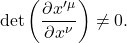
$\det\left(\frac{\partial x'^\mu}{\partial x^\nu}\right)\neq 0.$

At this stage, we have introduced no metric. We cannot yet calculate lengths, angles or elapsed proper time.

Also, the coordinate values $x^\mu$ themselves are generally not vector components: coordinate changes can be nonlinear or include translations.

2. A scalar is a number attached to an event

A scalar field assigns a number to each point:

$\phi=\phi(x).$

Its value at a particular event is independent of coordinates:

$\boxed{\phi'(x')=\phi(x).}$

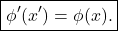
The function’s expression can change even though its value at the same point does not.

For example, in two dimensions,

$\phi(x,y)=x^2+y^2$

becomes, in polar coordinates,

$\phi'(r,\theta)=r^2.$

These are two expressions for the same field.

3. Coordinate displacements give the prototype of a contravariant vector

The chain rule gives

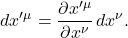
$dx'^\mu = \frac{\partial x'^\mu}{\partial x^\nu}\,dx^\nu.$

Schrödinger defines a contravariant vector as a quantity transforming this way:

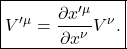
$\boxed{ V'^\mu = \frac{\partial x'^\mu}{\partial x^\nu}V^\nu. }$

A useful example is the tangent to a curve $x^\mu(s)$ :

$V^\mu=\frac{dx^\mu}{ds},$

where $s$ is a fixed curve parameter independent of the coordinate choice.

The vector belongs to a particular point. The Jacobian used to transform it is evaluated at that point.

4. Scalar derivatives give the prototype of a covariant vector

Now differentiate a scalar field:

$\partial_\mu\phi \equiv \frac{\partial\phi}{\partial x^\mu}.$

The chain rule gives

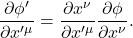
$\frac{\partial\phi'}{\partial x'^\mu} = \frac{\partial x^\nu}{\partial x'^\mu} \frac{\partial\phi}{\partial x^\nu}.$

Notice the inverse Jacobian, compared with the vector transformation law.

A covariant vector, or covector, therefore transforms as

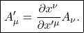
$\boxed{ A'_\mu = \frac{\partial x^\nu}{\partial x'^\mu}A_\nu. }$

Thus:

Object	Transformation factor
Vector $V^\mu$	$\partial x'^\mu/\partial x^\nu$
Covector $A_\mu$	$\partial x^\nu/\partial x'^\mu$

The different index positions record different transformation laws.

5. Their contraction is invariant

The change in a scalar between neighboring points is

$d\phi=\partial_\mu\phi\,dx^\mu.$

Written explicitly,

$d\phi = \frac{\partial\phi}{\partial x^0}dx^0 + \frac{\partial\phi}{\partial x^1}dx^1 + \frac{\partial\phi}{\partial x^2}dx^2 + \frac{\partial\phi}{\partial x^3}dx^3.$

Both factors change under a coordinate transformation, but their changes cancel:

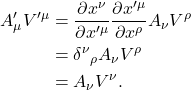
$\begin{aligned} A'_\mu V'^\mu &= \frac{\partial x^\nu}{\partial x'^\mu} \frac{\partial x'^\mu}{\partial x^\rho} A_\nu V^\rho\\ &=\delta^\nu{}_\rho A_\nu V^\rho\\ &=A_\nu V^\nu. \end{aligned}$

Therefore,

$\boxed{A_\mu V^\mu\text{ is a scalar}.}$

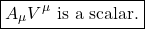
Geometrically, a covector takes a vector as input and returns a number. This pairing requires no metric.

6. Tensors generalize these transformation laws

A tensor has one transformation factor for each index. For example,

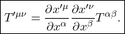
$\boxed{ T'^{\mu\nu} = \frac{\partial x'^\mu}{\partial x^\alpha} \frac{\partial x'^\nu}{\partial x^\beta} T^{\alpha\beta}. }$

A mixed tensor transforms as

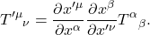
$T'^\mu{}_\nu = \frac{\partial x'^\mu}{\partial x^\alpha} \frac{\partial x^\beta}{\partial x'^\nu} T^\alpha{}_\beta.$

An array of numbers qualifies as a tensor because it obeys the appropriate transformation law.

A product such as

$T^{\mu\nu}=V^\mu W^\nu$

provides an example, although a general rank-two tensor need not factor into a single product.

7. Tensor algebra preserves coordinate independence

The chapter develops several operations:

Operation	Example	Result
Addition of tensors of the same type at the same point	$A^\mu+B^\mu$	A vector
Tensor product	$A^\mu B_\nu$	A mixed rank-two tensor
Contraction	$T^\mu{}_\mu$	A scalar
Symmetric part	$\frac12(T_{\mu\nu}+T_{\nu\mu})$	A symmetric tensor
Antisymmetric part	$\frac12(T_{\mu\nu}-T_{\nu\mu})$	An antisymmetric tensor

For example,

$T^\mu{}_\mu = T^0{}_0+T^1{}_1+T^2{}_2+T^3{}_3.$

Contraction pairs one upper index with one lower index. We cannot yet freely raise and lower indices, because that requires a metric.

Likewise, vectors at different points cannot yet be compared by parallel transport: we have not introduced a connection.

8. Why tensor equations are useful physical laws

Suppose

$S_{\mu\nu}=T_{\mu\nu}.$

Equivalently,

$S_{\mu\nu}-T_{\mu\nu}=0.$

Because tensor transformations are linear and homogeneous, a tensor whose components all vanish in one coordinate system vanishes in every coordinate system.

Consequently:

$\boxed{ \text{A tensor equation valid in one coordinate system remains valid in every coordinate system.} }$

This makes tensors a natural language for expressing coordinate-independent physical relationships. It does not determine which relationships are physically correct; dynamics must still supply that information.

9. The chapter’s final tool: recognizing a tensor indirectly

Schrödinger proves a useful converse.

If an array $S_{\mu\nu}$ satisfies

$S_{\mu\nu}V^\mu W^\nu = \text{a scalar}$

for every independently chosen pair of vectors $V^\mu,W^\nu$ , then $S_{\mu\nu}$ must transform as a covariant tensor.

The arbitrary vectors probe every component of the array. Requiring their contraction to be invariant forces the tensor transformation law.

One application is the identity tensor:

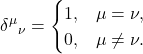
$\delta^\mu{}_\nu = \begin{cases} 1,&\mu=\nu,\\ 0,&\mu\neq\nu. \end{cases}$

It satisfies

$\delta^\mu{}_\nu V^\nu=V^\mu$

and has the same numerical components in every coordinate system.

Connection to your scalar Lagrangian question

We can now distinguish what geometry is needed for

$\mathcal L = \frac12\partial_\mu\phi\,\partial^\mu\phi -\frac12m^2\phi^2.$

Chapter I already gives us the scalar $\phi$ and covector $\partial_\mu\phi$ . But writing an upper derivative index requires a metric:

$\partial^\mu\phi = g^{\mu\nu}\partial_\nu\phi.$

Thus the kinetic term really means

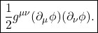
$\boxed{ \frac12g^{\mu\nu} (\partial_\mu\phi)(\partial_\nu\phi). }$

The metric supplies the missing structure needed to contract those two covectors. In Minkowski coordinates, $g^{\mu\nu}=\eta^{\mu\nu}$ , producing the time and spatial derivative terms we expanded earlier.

The central lesson of Chapter I: vectors and tensors describe local quantities without requiring a notion of distance. A connection and a metric add further capabilities later.

Next is Chapter II: Integrals, Densities, Derivatives, which asks how integration and differentiation behave when coordinates change.

Schrödinger’s Space-Time Structure – Chapter 1

No Comments Yet

Leave a Reply Cancel reply